Rent-seeking is any deliberate attempt to obtain rents, usually by political power, market power, influencing and using the law, or a combination of such means. Rent-seeking benefits no one, except the rent-seeker. It is a good idea to discourage rent-seeking, and some ideas about that are discussed below.
In the wonderful book The invisible hand? How market economies have emerged and declined since AD500, Bas van Bavel analyzes three examples of pre-industrial market economies: Iraq in the early Middle Ages, Italy in the high Middle Ages, and the Low Countries in the late Middle Ages and the early modern period. He analyzes that these societies thrived with dynamic and open markets, and how the growth of prosperity leads to the rise of new elites who accumulate assets, and how elites and privileged groups gradually tend to protect those assets, thus reducing dynamic and open markets. We can view this process as an increase in rent-seeking, which gradually leads to a decline of a society in the long run. With this in mind it is a good idea to pay attention to rent-seeking and to consider means to discourage it.
Katharina Pistor is the author of the book “The code of capital”. The subtitle is “How the law creates wealth and inequality”. This book describes how a simple object, an idea, or a promise to pay can be transformed into an asset that creates wealth. By doing this she explains how capital is created by lawyers.
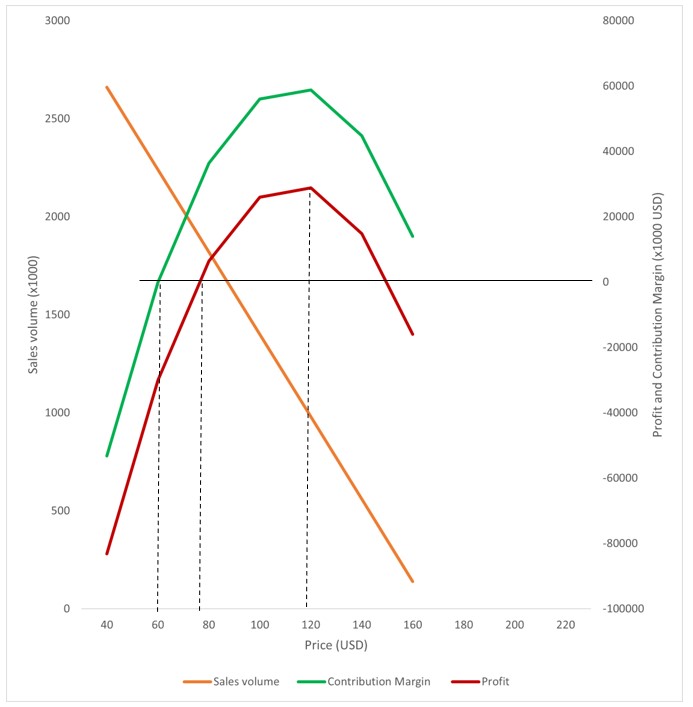
In figure 1 the contribution margin is the contribution to cover fixed costs, and is calculated as revenues minus variable costs (for the precise numbers see year-2021 in table 1 below). Many firms use the contribution margin as base for pricing because it is often difficult and rather arbitrary to allocate fixed costs among products. The dashed vertical lines in figure 1 define three important prices for the supplier. The left line (price = 60) is the ‘minimum price’ where the contribution margin is zero. The middle dashed line (price = 80) is the ‘required price’ where the contribution margin is equal to fixed costs. The third dashed line (price = 103) is the ‘maximum price’ which optimizes the contribution margin and profit. Any price above this maximum reduces profit, due to price elasticity of demand. Even a monopolist will charge this maximum price, unless the monopolist is able to reduce the price elasticity of demand, as discussed below in the section ‘Bargaining power and price elasticity of demand’.
Another way of looking at figure 1 is that the minimum price and the maximum price define the bargaining space for a supplier. An example is the price which a hotel chain can charge for a room. In January demand is often so low that the hotel chain cannot charge more than the minimum price. If even the minimum price is not feasible the hotel may close down temporarily because the price does not even cover variable costs. In the peak season or during special events (e.g. a large trade fair) the hotel chain can charge the maximum price. The average price over the year must at least equal the required price in order to be a profitable business. If not, the hotel chain will not continue for a long time, because shareholders may sell their shares, banks may cut credit lines and it is unlikely that new investors are interested.
Bargaining power and the price elasticity of supply
If supply is flexible and fully adjusts to demand the price elasticity of supply is > 1, and no supplier can increase price more than the competition. In terms of figure 1 the average price over the year will be equal to the required price. Consequently there can be no economic rents because any higher price will be driven down by competition (see the blog How to calculate rents).
To summarize: a condition for economic rents is that the price elasticity of supply < 1.
Bargaining power and price elasticity of demand
Figure 2 is based on the same numbers as figure 1, with one important difference: the price elasticity of demand is much lower in figure 2. If the price = 100 the price elasticity of demand in figure 1 equals -1.5 while it is -0.5 in figure 2.
A monopolist may charge a price of 113 USD in figure 1, while the monopolist may charge 176 USD in figure 2. As a result the maximum profit equals almost 30 million USD in figure 1 while it is 131 million USD in figure 2. Therefore it is very attractive for a monopolist to reduce the price elasticity of demand as much as possible. If the customer is unable to use another vendor without substantial switching costs this is called a vendor lock-in. Less extreme examples of methods to reduce price elasticity of demand are: product differentiation and brand name.
One example of a vendor lock-in is Apple: the closed ecosystem of Apple products makes it quite unattractive for a customer to switch to another product. Consequently Apple can charge higher prices than competitors.
The most extreme example of figure 2 is a pharmaceutical product, with a patent, and which can cure a life-threatening disease. In such a case the price elasticity of demand will be close to zero and consequently the supplier can charge an extremely high price.
Bargaining power and inflation
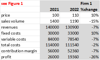
If a supplier has strong bargaining power it is easier to pass-through any cost increase, and this is illustrated by comparing firms in Table 1 and Table 2.
Table 1 Effect of 10% inflation for firm with weak bargaining power (sales volume = 3500-21*price)
Table 2 Effect of 10% inflation for firm with strong bargaining power (sales volume = 3500-12*price)
Due to inflation, both firms face an increase in their fixed and variable costs of 10%. Both firms respond by raising the sales price by 10%. However, for firm 1 the profit goes down by 26%, while for firm 2 the profit increases by 1%.
Definitions
Contribution margin: sales minus variable costs. This is the contribution to cover fixed costs.
Contribution margin ratio: (sales minus variable costs) / sales, for example (100-80)/100 = 20%. This means that 20% of sales revenues is used to cover fixed costs.
Markup: Sales / costs – 1, for example 100/80 – 1 = 1.25 – 1 = 25%. This is the percentage which is added to costs in order to calculate the sales price.
Rents can be measured as a surplus cash flow, see table1 and figure1 below.
Revenues (sales)
–
Cost of Goods Sold (COGS)
–
Selling, General & Administrative costs (SG&A)
–
Research and Development costs (R&D)
–
Investments (Capex expenses)
+
Depreciation (to adjust for the depreciation costs in COGS, because investments are fully expensed as cash flow)
–
normal Return On Investment (the return in competitive markets, which is the required return for long-term continuity of the firm)
=
surplus cash flow = rents
table1
For this calculation I use data in the operational section of the Statement of cash flows in Annual reports. The normal return on investment is discussed in the blog A normal return .
Rents in one year may be an incident, e.g. temporary scarcity due to a bad harvest or a war. It is the persistent rents which are relevant as the result of possession of scarce or exclusive assets. A proxy for persistent rents is the minimum of rents in five years. For example: if rents in the last five years were 26, 28, 22, 30, 32 % of revenues, then the minumum % in the last five years was 22%. That is: proxy for persistent rents = 22% of revenues.
Figure1 Rents as surplus cash flow
The method above is explained in detail in my paper in the Cambridge Journal of Economics, volume 47, issue 4, July 2023, https://doi.org/10.1093/cje/bead025